The Data Scientist’s Guide to Probability Distributions

Probability Basics

Probability is the foundation of statistical analysis and data science. It represents the likelihood of an event occurring. The formula for probability is:

where:

$P$ is the probability of the event,

$m$ is the number of favorable outcomes,

$n$ is the total number of possible outcomes.

Common Probability Distributions

Uniform Distribution
All outcomes are equally likely. For a discrete uniform distribution:

The formula for the probability density function (PDF) of a continuous uniform distribution for a random variable $X$ between $a$ and $b$ is:

$$f(X=x) = \frac{1}{b-a}, \quad a \leq x \leq b$$

where $n$ is the number of possible outcomes.

Example: Choosing a random number between 1 and 6 (inclusive), where any real number in this range is equally likely.

The random variable $X$ is uniformly distributed between $1$ and $b=6$. Using the PDF formula:

$$f(x)= \frac{1}{b-a}, \quad a \leq x \leq b$$

Substituting $a=1$ and $b=6$:

$$f(x)= \frac{1}{6-1} = \frac{1}{5}$$

This means that the probability density (not the probability) of any point $x$ in the interval $[1, 6]$ is $0.2$ or $\frac{1}{5}$.

For a continuous distribution, the total probability across the interval equals 1, but the probability of a specific point $x$ (like exactly $x=3$) is $0$ because continuous distributions deal with ranges.

Normal Distribution
The bell-shaped curve commonly used in statistics. The probability density function (PDF) is:

where:

$\mu$ is the mean,

$\sigma$ is the standard deviation.

Example: Heights of people in a population are typically normally distributed.

Binomial Distribution
The probability of $k$ successes in $n$ trials, where each trial has a success probability $p$, is given by:

Example: The probability of flipping a coin 10 times and getting exactly 6 heads when $p = 0.5$

Poisson Distribution
Models the number of events occurring in a fixed interval of time or space. The formula is:

where $\lambda$ is the average rate of occurrence.

Example: The number of emails received per hour when the average is 5 emails/hour.

Key Concepts in Probability

Bayes' Theorem
A fundamental theorem used to update probabilities based on new evidence:

Expected Value
The mean of a random variable is given by:

or for continuous variables:

Variance and Standard Deviation
Variance is a measure of how spread out the values are:

The standard deviation is:

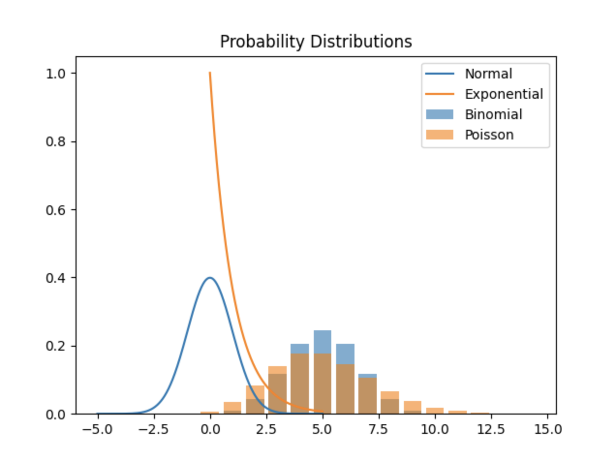
Visualizing Distributions in Python

Here’s a Python snippet to visualize distributions using matplotlib:


import numpy as np
import matplotlib.pyplot as plt
from scipy.stats import norm, binom, expon, poisson

# Normal Distribution
x = np.linspace(-5, 5, 1000)
plt.plot(x, norm.pdf(x, loc=0, scale=1), label="Normal")

# Binomial Distribution
n, p = 10, 0.5
x_binom = np.arange(0, n+1)
plt.bar(x_binom, binom.pmf(x_binom, n, p), alpha=0.6, label="Binomial")

# Exponential Distribution
x_exp = np.linspace(0, 5, 1000)
plt.plot(x_exp, expon.pdf(x_exp, scale=1), label="Exponential")

# Poisson Distribution
x_poisson = np.arange(0, 15)
plt.bar(x_poisson, poisson.pmf(x_poisson, mu=5), alpha=0.6, label="Poisson")

plt.legend()
plt.title("Probability Distributions")
plt.show()