Confidence Intervals and Hypothesis Testing Made Simple
1. What are Confidence Intervals?
A confidence interval ($CI$) is a range of values, derived from a sample statistic, that is used to estimate an unknown population parameter. The interval has an associated confidence level, which quantifies the level of confidence that the parameter lies within the interval.
The formula for a confidence interval is:
$$CI = \bar{x} \pm Z \cdot \frac{\sigma}{\sqrt{n}}$$
Where:
- $\bar{x}$ is the sample mean.
- $Z$ is the Z-value (critical value from the standard normal distribution, depending on the confidence level).
- $\sigma$ is the population standard deviation (or sample standard deviation if the population standard deviation is unknown).
- $n$ is the sample size.
Example:
If we sample 100 people from a population and calculate their average height to be 170 cm with a population standard deviation of 5 cm, the 95% confidence interval for the mean height would be:
$$CI = 170 \pm 1.96 \cdot \frac{5}{\sqrt{100}}$$
This means the true mean height of the population has a 95% chance of lying within this range.
2. Understanding Hypothesis Testing
Hypothesis testing is a statistical method used to determine if there is enough evidence in a sample of data to support or reject a hypothesis about a population parameter.
The two main hypotheses are:
- Null Hypothesis ($H_0$): This hypothesis assumes no effect or no difference. For example, it could state that the average height in a population is equal to 170 cm.
- Alternative Hypothesis ($H_1$): This hypothesis suggests that there is an effect or difference. For example, it could state that the average height is not equal to 170 cm.
The hypothesis test involves calculating a test statistic (such as the t-statistic or z-statistic) and comparing it to a critical value, which is determined based on the significance level ($\alpha$). The most common significance level is 0.05.
The formula for a z-test statistic is:
$$z = \frac{\bar{x} - \mu}{\frac{\sigma}{\sqrt{n}}}$$
Where:
- $\bar{x}$ is the sample mean.
- $\mu$ is the population mean under the null hypothesis.
- $\sigma$ is the population standard deviation.
- $n$ is the sample size.
Example:
If we have a sample mean of 172 cm, a population mean of 170 cm, a population standard deviation of 5 cm, and a sample size of 100, the z-test statistic would be:
$$z = \frac{172 - 170}{\frac{5}{\sqrt{100}}}$$
If the z-value exceeds the critical value (for a two-tailed test at a 0.05 significance level, the critical z-value is approximately 1.96), we reject the null hypothesis.
3. Types of Errors in Hypothesis Testing
- Type I Error: Rejecting the null hypothesis when it is actually true (false positive).
- Type II Error: Failing to reject the null hypothesis when it is false (false negative).
4. Example with Visualization using numpy
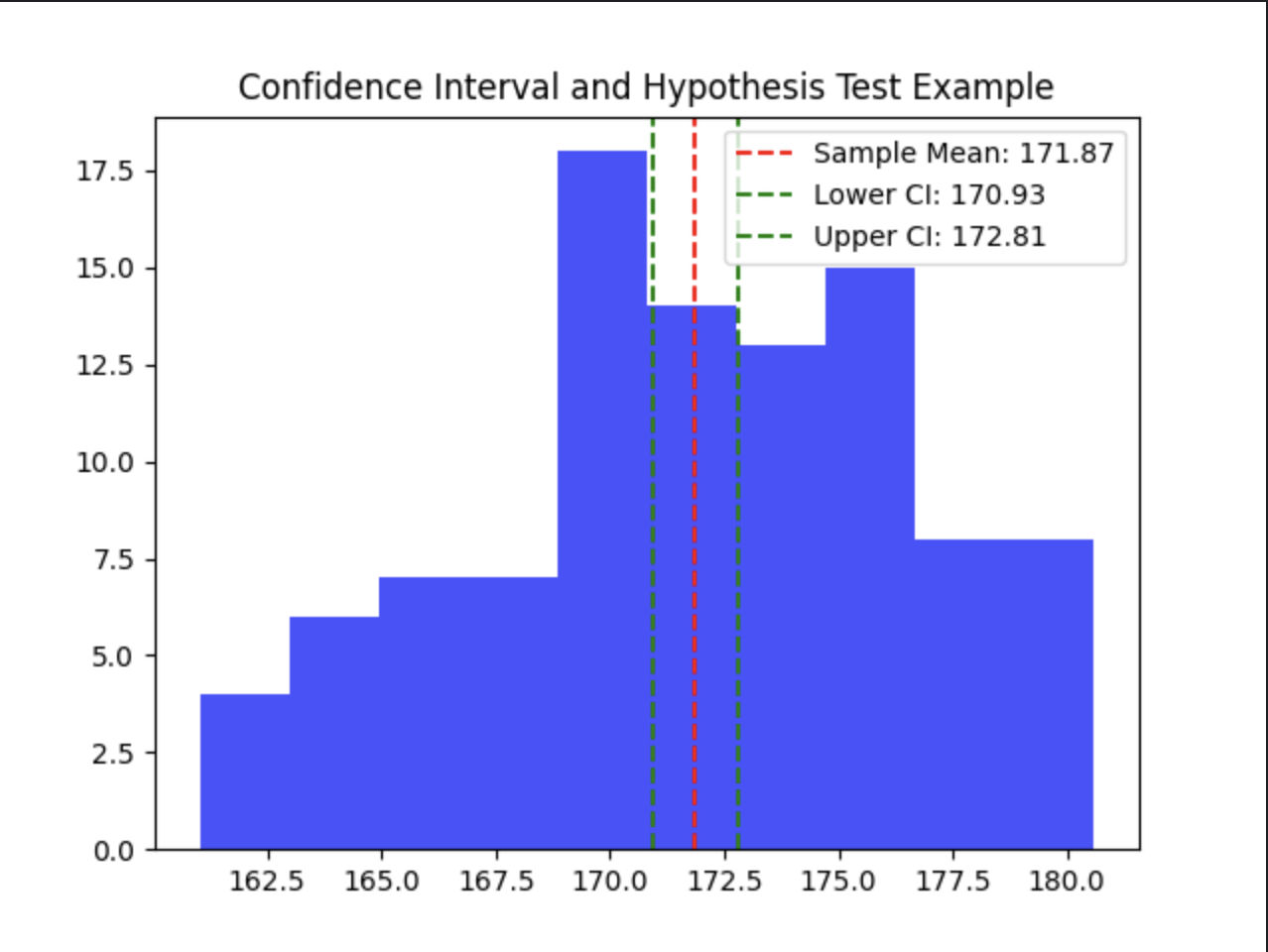
Let's consider a situation where we have a sample data set, and we want to test the hypothesis that the population mean is 170 cm. We will calculate the confidence interval and perform a hypothesis test using .
import numpy as np
import matplotlib.pyplot as plt
from scipy import stats

# Sample data: heights of 100 people
sample_data = np.random.normal(172, 5, 100)  # mean = 172, std dev = 5, n = 100

# 1. Confidence Interval Calculation
sample_mean = np.mean(sample_data)
sample_std = np.std(sample_data)
n = len(sample_data)
confidence_level = 0.95
Z = stats.norm.ppf(1 - (1 - confidence_level) / 2)

margin_of_error = Z * (sample_std / np.sqrt(n))
confidence_interval = (sample_mean - margin_of_error, sample_mean + margin_of_error)

# 2. Hypothesis Testing (z-test)
population_mean = 170
z_score = (sample_mean - population_mean) / (sample_std / np.sqrt(n))

# Plotting the distribution and confidence interval
plt.hist(sample_data, bins=10, alpha=0.7, color='blue')
plt.axvline(sample_mean, color='red', linestyle='dashed', label=f'Sample Mean: {sample_mean:.2f}')
plt.axvline(confidence_interval[0], color='green', linestyle='dashed', label=f'Lower CI: {confidence_interval[0]:.2f}')
plt.axvline(confidence_interval[1], color='green', linestyle='dashed', label=f'Upper CI: {confidence_interval[1]:.2f}')
plt.title('Confidence Interval and Hypothesis Test Example')
plt.legend()
plt.show()

print(f"Confidence Interval: {confidence_interval}")
print(f"Z-score for Hypothesis Testing: {z_score:.2f}")

In this example:
- We generate random sample data based on a normal distribution.
- Calculate the confidence interval for the sample mean.
- Perform a z-test to determine if the sample mean significantly differs from the hypothesized population mean.
5. Conclusion
Confidence intervals provide a range of plausible values for a population parameter, while hypothesis testing helps to make decisions or inferences about population parameters based on sample data. Understanding these two concepts is crucial for data scientists and researchers when drawing conclusions from data.
Tags: Confidence Intervals, Data Science, Hypothesis Testing, P-value, Probability, Sample Data, Statistical Inference, Statistics, Type I Error, Type II Error, Z-test


